${\displaystyle \left[{\begin{array}{c}{\frac {d\omega _{r}}{dt}}\\{\frac {di_{a}}{dt}}\end{array}}\right]=\left[{\begin{array}{cc}A_{11}&A_{12}\\A_{21}&A_{22}\end{array}}\right]\left[{\begin{array}{c}\omega _{r}\\i_{a}\end{array}}\right]+\left[{\begin{array}{cc}B_{11}&B_{12}\\B_{21}&B_{22}\end{array}}\right]\left[{\begin{array}{c}u_{1}\\u_{2}\end{array}}\right]}$

${\displaystyle {\mathcal {L}}\{af(t)+bg(t)\}=aF(s)+bG(s)}$

${\displaystyle {\mathcal {L}}\{f'(t)\}=sF(s)-f(0)}$

${\displaystyle \Omega (s)={\frac {()V_{a}(s)+()T_{L}(s)}{s+()}}}$

${\displaystyle \left.{\frac {\Omega (s)}{V_{a}(s)}}\right|_{T_{L}(s)=0}=?}$

${\displaystyle \left.{\frac {\Omega (s)}{T_{L}(s)}}\right|_{V_{a}(s)=0}=?}$

${\displaystyle v_{a}(t)=V_{a}u(t)}$

${\displaystyle \omega _{r}(t)={\mathcal {L}}^{-1}\left\{{\frac {\Omega (s)}{V_{a}(s)}}V_{a}(s)\right\}}$

---

(1) ${\displaystyle T_{e}-T_{L}=J{\frac {dw_{r}}{dt}}+B_{m}w_{r}}$

(2) ${\displaystyle v_{a}=r_{a}i_{a}+L_{aa}{\frac {di_{a}}{dt}}+k_{v}w_{r}}$

(3) ${\displaystyle T_{e}=k_{T}i_{a}}$

Solve equations (1) and (2) for ${\displaystyle {\frac {dw_{r}}{dt}}}$ and ${\displaystyle {\frac {di_{a}}{dt}}}$.

${\displaystyle {\frac {dw_{r}}{dt}}={\frac {1}{J}}\left[-B_{m}w_{r}+k_{t}i_{a}-T_{L}\right]}$

${\displaystyle {\frac {di_{a}}{dt}}={\frac {1}{L_{aa}}}\left[-k_{v}w_{r}-r_{a}i_{a}+V_{a}\right]}$

${\displaystyle \left[{\begin{array}{c}{\frac {d\omega _{r}}{dt}}\\{\frac {di_{a}}{dt}}\end{array}}\right]=\left[{\begin{array}{cc}-{\frac {B_{m}}{J}}&{\frac {k_{T}}{J}}\\-{\frac {k_{v}}{L_{aa}}}&-{\frac {r_{a}}{L_{aa}}}\end{array}}\right]\left[{\begin{array}{c}\omega _{r}\\i_{a}\end{array}}\right]+\left[{\begin{array}{cc}-{\frac {1}{J}}&0\\0&{\frac {1}{L_{aa}}}\end{array}}\right]\left[{\begin{array}{c}T_{L}\\V_{a}\end{array}}\right]}$

${\displaystyle T_{e}-T_{L}=B_{m}\Omega _{r}}$

${\displaystyle V_{a}=r_{a}I_{a}+k_{v}\Omega _{r}}$

${\displaystyle T_{e}=k_{T}I_{a}}$

${\displaystyle T_{e}-T_{L}=J{\frac {dw_{r}}{dt}}+B_{m}w_{r}}$

${\displaystyle v_{a}=r_{a}i_{a}+k_{v}w_{r}}$

${\displaystyle T_{e}=k_{T}i_{a}}$

Combine equations (1)-(3) to eliminate ${\displaystyle i_{a}}$. First solve (1) and (3) for ${\displaystyle i_{a}}$

${\displaystyle i_{a}={\frac {1}{k_{T}}}\left(J{\frac {d\omega _{r}}{dt}}+B_{m}\omega _{r}+T_{L}\right)}$

Then substitute the result into (2).

${\displaystyle v_{a}={\frac {r_{a}}{k_{T}}}\left(J{\frac {d\omega _{r}}{dt}}+B_{m}\omega _{r}+T_{L}\right)+k_{v}\omega _{r}}$

Convert the resulting equation to the frequency domain through application of Laplace transforms. Note that we choose the capital form of ${\displaystyle \omega }$ (${\displaystyle \Omega }$), when in the frequency domain. Also, it is safe to assume ${\displaystyle \omega _{r}(t)=0}$.

${\displaystyle V_{a}(s)={\frac {r_{a}}{k_{T}}}\left(Js\Omega _{r}(s)+B_{m}\Omega _{r}(s)+T_{L}(s)\right)+k_{v}\Omega _{r}(s)}$

Solving the resulting equation for ${\displaystyle \Omega _{r}(s)}$ yeilds

${\displaystyle \Omega _{r}(s)={\frac {{\frac {k_{T}}{Jr_{a}}}V_{a}(s)-{\frac {1}{J}}T_{L}(s)}{s+{\frac {B_{m}r_{a}+k_{T}k_{v}}{Jr_{a}}}}}}$

Finally, solve the above equation for the transfer functions

${\displaystyle \left.{\frac {\Omega _{r}(s)}{V_{a}(s)}}\right|_{T_{L}(s)=0}={\frac {\frac {k_{T}}{Jr_{a}}}{s+{\frac {B_{m}r_{a}+k_{T}k_{v}}{Jr_{a}}}}}}$

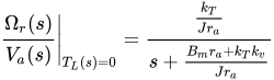
and

${\displaystyle \left.{\frac {\Omega _{r}(s)}{T_{L}(s)}}\right|_{V_{a}(s)=0}={\frac {-{\frac {1}{J}}}{s+{\frac {B_{m}r_{a}+k_{T}k_{v}}{Jr_{a}}}}}}$

Using the first transfer function above, solve for ${\displaystyle \omega _{r}(t)}$ given ${\displaystyle v_{a}(t)=V_{a}u(t)}$. In other words, solve the following

${\displaystyle \omega _{r}(t)={\mathcal {L}}^{-1}\left\{{\frac {\Omega (s)}{V_{a}(s)}}\cdot V_{a}(s)\right\}}$.

${\displaystyle \omega _{r}(t)={\mathcal {L}}^{-1}\left\{{\frac {\frac {k_{T}}{Jr_{a}}}{s+{\frac {B_{m}r_{a}+k_{T}k_{v}}{Jr_{a}}}}}\cdot {\frac {V_{a}}{s}}\right\}}$

We use a Laplace transform table to look up the transform for an exponential approach

${\displaystyle {\mathcal {L}}^{-1}\left\{{\frac {\alpha }{s(s+\alpha )}}\right\}=\left(1-e^{-\alpha t}\right)\cdot u(t)}$

then if we let

${\displaystyle \alpha ={\frac {B_{m}r_{a}+k_{T}k_{v}}{Jr_{a}}}}$

we can express ${\displaystyle \omega _{r}(t)}$ as

${\displaystyle \omega _{r}(t)={\mathcal {L}}^{-1}\left\{{\frac {k_{T}V_{a}}{B_{m}r_{a}+k_{t}k_{v}}}\cdot {\frac {\alpha }{s(s+\alpha )}}\right\}={\frac {k_{T}V_{a}}{B_{m}r_{a}+k_{t}k_{v}}}\left(1-e^{-\alpha t}\right)\cdot u(t)}$.

Given

${\displaystyle \omega _{r}(t)=\omega _{r,ss}\left(1-e^{-t/\tau _{m}}\right)}$

we have

${\displaystyle \omega _{r,ss}={\frac {k_{T}V_{a}}{B_{m}r_{a}+k_{t}k_{v}}}}$

and

${\displaystyle \tau _{m}={\frac {Jr_{a}}{B_{m}r_{a}+k_{T}k_{v}}}}$

(1) ${\displaystyle k_{T}i_{a}-T_{L}=J{\frac {d\omega _{r}}{dt}}+B_{m}\omega _{r}}$

(2) ${\displaystyle v_{a}=r_{a}i_{a}+k_{v}\omega _{r}}$

(3) ${\displaystyle v_{a}=K_{1}+K_{2}\cos(\omega _{e}t)}$

(4) ${\displaystyle \omega _{r}=\omega _{ro}+A\cos(\omega _{e}t+\phi )}$

Solving equation (1) for ${\displaystyle i_{a}}$ and substituting into equation (2) results in

${\displaystyle v_{a}={\frac {r_{a}}{k_{T}}}\left(J{\frac {d\omega _{r}}{dt}}+B_{m}\omega _{r}\right)+k_{v}\omega _{r}}$

Simplifying

${\displaystyle v_{a}={\frac {Jr_{a}}{k_{T}}}{\frac {d\omega _{r}}{dt}}+{\frac {B_{m}r_{a}+k_{T}k_{v}}{k_{T}}}\omega _{r}}$

Now equations (3) and (4) can be substituted into the above equation to produce

${\displaystyle K_{1}+K_{2}\cos(\omega _{e}t)=-{\frac {Jr_{a}}{k_{T}}}A\omega _{e}\sin(\omega _{e}t+\phi )+{\frac {B_{m}r_{a}+k_{T}k_{v}}{k_{T}}}\left(\omega _{ro}+A\cos(\omega _{e}t+\phi )\right)}$

Applying some trigonometry the above can be rewritten as

${\displaystyle K_{1}+K_{2}\cos(\omega _{e}t)={\frac {B_{m}r_{a}+k_{T}k_{v}}{k_{T}}}\omega _{ro}+{\sqrt {\left({\frac {Jr_{a}\omega _{e}}{k_{T}}}A\right)^{2}+\left({\frac {B_{m}r_{a}+k_{T}k_{v}}{k_{T}}}A\right)^{2}}}\cos(\omega _{e}t)}$

${\displaystyle \omega _{r0}={\frac {k_{T}K_{1}}{B_{m}r_{a}+k_{T}k_{v}}}}$

${\displaystyle A={\sqrt {\frac {(k_{T}K_{2})^{2}}{(Jr_{a}\omega _{e})^{2}+(B_{m}r_{a}+k_{T}k_{v})^{2}}}}}$

${\displaystyle J={\frac {1}{r_{a}\omega _{e}}}{\sqrt {\left({\frac {k_{T}K_{2}}{A}}\right)^{2}-(B_{m}r_{a}+k_{T}k_{v})^{2}}}}$

${\displaystyle \left|e_{ab}\right|={\sqrt {3}}\,\omega _{r}\lambda _{m}^{'}}$

The Fourier series of a 2π-periodic function ƒ(x) that is integrable on [−π, π], is given by

${\displaystyle {\frac {a_{0}}{2}}+\sum _{n=1}^{\infty }\,[a_{n}\cos(nx)+b_{n}\sin(nx)]}$

where

${\displaystyle a_{n}={\frac {1}{\pi }}\int _{-\pi }^{\pi }f(x)\cos(nx)\,dx,\quad n\geq 0}$

and

${\displaystyle b_{n}={\frac {1}{\pi }}\int _{-\pi }^{\pi }f(x)\sin(nx)\,dx,\quad n\geq 1}$

In question 2, you are being asked to find the fundamental component of the fourier series of the functions vas, vbs, and vcs. The fundamental component is the component with the lowest freqency, specifically:

${\displaystyle v_{as}(\theta _{r})\approx {\frac {a_{0}}{2}}+a_{1}\cos(\theta _{r})+b_{1}\sin(\theta _{r})}$

To find the coefficients an and bn from the equations above, the integral must be broken down into the sum of integrals over continuous regions.

${\displaystyle {\begin{array}{l}\int \limits _{-\pi }^{\pi }f\,dx=\int \limits _{-\pi }^{-{\frac {2\pi }{3}}}f\,dx\,+\int \limits _{-{\frac {2\pi }{3}}}^{-{\frac {\pi }{3}}}f\,dx\,+\int \limits _{-{\frac {\pi }{3}}}^{0}f\,dx\,\\\qquad \qquad \qquad +\int \limits _{0}^{\frac {\pi }{3}}f\,dx\,+\int \limits _{\frac {\pi }{3}}^{\frac {2\pi }{3}}f\,dx\,+\int \limits _{\frac {2\pi }{3}}^{\pi }f\,dx\end{array}}}$

${\displaystyle T_{e}=-3L_{B}\{i_{as}^{2}\sin \left(6\theta _{rm}\right)+i_{bs}^{2}\sin \left[6\left(\theta _{rm}-20\,^{\circ }\right)\right]+i_{cs}^{2}\sin \left[6\left(\theta _{rm}+20\,^{\circ }\right)\right]\}}$

${\displaystyle \left[{\begin{array}{ccc}\;\,&\;\,&\;\,\\&&\\&&\end{array}}\right]\left[{\begin{array}{c}e_{as}\\e_{bs}\\e_{cs}\end{array}}\right]=\left[{\begin{array}{c}e_{ab}\\e_{cb}\\0\end{array}}\right]}$